WARNING ; very technical.
The entire methodology relies on a simple principle;
REVERSE INFERENCE
Imagine watching the mind to see how it responds to stimuli as you jab the host with an electrical prod. Did the article appear at the top? Probably not.
This is more akin to simulating MRI scans; far less violent, but we still watch what happens from recorded stimuli. More akin to testing outcomes from many matching tests; simulating pockets of time. We see 50 ways to perform a task and choose the best option between them all and then scale based on the various learn rates to train them all at once based on a large series of factors.
Sim V5 expert models were trained using traditional cosine methods in Kohya_SS using ADAfactor for direct conformity from point A to B to create the foundation experts interpolated into Beatrix V1 reverse inference interpolation model experiment weights.
NOT to be confused with BeatriXL - they are very different models. Beatrix is a 600 layer interpolation system that weighs nearly 70 gigs of vram to inference when the experts are all loaded into memory. It's inferenced using the T5XL or the T5XXL unchained, but the unchained one isn't ready. It produces anchor point positions based on a few factors; context window, vector shift, timestep distilled... y'know what this thing is insanely complicated. I still haven't finished my full paper on it yet.
Well it turns out, I don't need such an elaborate schema to make it happen for the sequel, now that Beatrix herself is operational. Beatrix's interpolation encoder is capable of interpolating at a rate of nearly 15x standard optimization capability when it comes to standard linear interpolation math, but there's some room for error. It does not climb a stack for recursion and it does not divide, it simply operates on the standard linear layers.
That's a 1,500% speed increase on interpolation math over the algorithmic methods I tested to direct model to model tensor predict. This is expected behavior, but I never expected such a large speed boost. I expected maybe a 4x or 10x. 15x is just a tip of the iceberg. This methodology can essentially distill lerp optimization into models, which wasn't the goal but it happened. I just wanted it to guess the specialized anchor point positions based on which expert model is necessary to use at which time, but we take byproducts.
You can see this speed if you generate images with the distilled diffusion decoded variation OmegaV0001; where you see the outcome literally cascade shifts over time autonomously. The outcome on nearly no steps shows that it learned a seriously high amount of data with very few steps and very little time required to create it due to the way the anchorpoints were injected and distilled into PonySim.
I did some research into the model "stable cascade" and saw it has a similar lerp concept as Beatrix, but it's not using the same principles, so I didn't gain much from it.
I'm going to describe to you the process of how the 600 layer Beatrix was trained now, as the process worked in classifiers, diffusion, and now entirely different types of encoder/decoder setups like CLIP, and there are even hints of it working from nearby researchers such as Felldude (different process similar principle, full credit to Felldude on this utilization as it's definitely divergent) with the SDXL VAE.
I'll get into detail about how the SDXL interpolation and distillation happened in the future when I have a bit more time to write articles. My time is quite limited these days.
Understanding The Process
This is a combination of training methods combined into one process that works like a cascading storm to teach models at seemingly impossible rapid speeds.
Methodology
SURGE is a combination of experience and math
We don't just build a gradient shift, we build a full ocean and simulate the wave.
We shift EVERYTHING along the model in intelligent ways, so it needs LESS changes with LESS optimizer updates and LESS training.
That way we don't NEED to run 50,000 images to get one result, we run one image in 50,000 ways to get all the results.
faster, is mastery.
a model which performs faster has mastered a task in the desired route, but that doesn't necessarily mean the data is correct.
faster often means skipping or zeroed or completely bypassed, which is identified in the interpolation process.
in Surge, we don't CARE if it's accurate. we aren't here to JUDGE accuracy of the outcome, that's not our task. Our task is to make the most optimal route from point A to B to C to D to E.
slower, is a knotted memory.
we want to smooth all of those out, we don't want knots, we want conformity and clean cohesion.
your banana doesn't need a box full of christmas lights to unroll for a single image, we want a nice clean lined up organized box that can be set out on display.
teacher / student process
our methodology is direct teacher / student interpolation, where either a second model as an expert is used, or the same model is used and forcefully interpolated using gathered neural feature data.
lerp the neurons and and force the hidden layers and attention heads to conform
the neurons are often the easy part, as you can force the neurons to be A or B, however the regulation systems in these models are often not the most conformist of them.
hidden layers must be conditioned and not destroyed, or the model will lose it's own cohesion.
interpolating between hidden layers is hazardous, so they must naturally learn to conform, or you'll end up with some of my byproduct trains on huggingface for the early interpolated SDXLs, where they generate some stuff well but the rest cascade fails.
4d interpolation of the attention heads
gathering the data allows us to build a 4d tensor of the attention heads and the ways they like to travel. we cannot see all the training as there's simply too much, and inflating this data would require a super computer subset to see it all
watching the attention heads is CRUCIAL. if you do not shift the model's attention carefully in line with the changes, the model will simply fail.
conforming the hidden layers in very small gradient nudges manually - only when needed
it has to be changed, so we update them using a vpred style trajectory loss - which the identical formula to vpred can be used based on gradient shifts of the hidden layers themselves with very, very, very low learn rate divided by how many layers of interpolation you're currently trying to mask into it.
essentially
We IDENTIFY the shared anchor points of interest between both models, where they both understand the topics using multiple checks and multiple seeds for identification.
We TARGET both using those anchor points for learning based on direct differences, and adjusting learning rates based on direct similarities.
We REPLACE neuron responses - we don't just conform the neurons, we find the pattern and replace the entire response with the desired effect and then test it.
We LERP the layers each at a time, manually, to ensure the interior of the model follows it's own rules along the chain based on the found data - and determine the difference between those ground data truths and the outcomes of the tests.
We HEAVILY adjust learn rate in the traditional sense at runtime - allowing us to make full use of standard learn rate systems and their optimizations whenever possible.
Dynamic Layer-difference based Learn Rate
In surge training, every layer has it's own learn rate based on the interpolated values, the differences between the teacher/student models, and the target features generated from the training data.
So for example; say you have a picture of a chicken. Your teacher model has a perfect understanding of the chicken, so you can get a fair and repeatable neural map of where the chicken is on that seed, and each iterative seed provides a similar map in some location within the model itself.
We target SLOW zones for learning. Slow zones are often points of difference that like to travel other routes, which means they are knotted. We need to be careful around those, so we need to test the individual layers with slow zones using not only the data used, but randomly sampled laion dataset flavors to find the culprit target flavor travel zones. Once identified we can use the information to skip past the information.
Inferencing only one layer is rapid, but the distilled flavors must be cached ahead of time or running it on the whole model will take too long. This is a model-to-model process and will likely require additional setup time for more types of models.
We increase learn rate for zones that have high differences. Those zones where we can say "okay so, you are having trouble here," scream that we need additional learning and additional mastery here. So, we can safely automatically distill a series of checks on layers above this layer here for the layer injection and testing, then run that singular layer a few thousand times nearly instantly, and determine the most optimal route for learning this information.
Phase 1; the data
This part is crucial, as if you're training nothing useful the model will learn nothing useful.
The Teachers
Choosing good teachers matters. You can choose the base trained weights of say SDXL or choose something like Pony. It doesn't matter as long as it fits within the matching model paradigm you set up, since this current process here does not allow for cross-model lerp learning... yet.
The teachers are to remain frozen. They do not learn; the student model needs to learn.
The amount of teachers doesn't matter. You just need to distill the outputs of the teachers in the correct way anchor point identification method to learn the correct neuron maps.
Raw Data
Choose the data that your model will understand. Whether it be images, audio, video, captions, whatever.
Already Trained Data Adapting
So say you have a lora that you want to train into a different model.
Hook the lora to your checkpoint and use that as a teacher model.
To make this data, you have to inference the model itself and generate the data using hooks into the model; akin to reverse engineering the model itself.
Distilling Flavors
This training method requires single layer modifications, so the models must be inferenced each epoch based on a certain amount of prompts. This can be scaled upward, or downward. In my case with OmegaV0001, I distilled hundreds of millions of these ahead of time, which allowed the first epoch of OmegaV0001 to train in almost zero time.
Phase 2; the setup
The data - is not the data you think it is.
An interpolation feature is a tensor map consisting of;
each layer:
the input datas, shapes, and or masks
the data is often a tensor picture and rich clip vectors
exact shapes for input and output
These are much less important but very useful for verification and gating
the activated neurons and their order
this is a lot of data, so you can extrapolate the difference of many and concatenate this - otherwise you'll end up with a traditional optimizer up to 50x the size of the model while training
the output data, shapes, and or masks
You need to end up with a rich set of datas.
the amount of time it took to get through this layer
Setting up the data can be very time consuming. It's essentially more than half of the process; as you're essentially inferencing two models over and over.
You want to gather all of the data from each layer from a series of images paired with their captions, using whatever clips you want to use as the catalyst, or whatever else you plan to use to send the information into the model or models you plan to use as teachers.
Phase 3; the training
Reusable Configurations
Shock Rate
Set to about 5
This determines how much you're willing to damage the model before it repairs, in this case 5 would multiply the steps internally for smoothing.
Smooth Rate
Set to inverse sq root of pi; 0.5641895835
This determines how much it's willing to learn based on how shocked the layer is, as a multiplier.
Steps
How many steps you're willing to make through the model, you generally only need one per image per epoch - and the steps can be very time consuming if you don't optimize using pytorch.
Batch Size
This is how many images to run through the system before it updates the weights and shifts the optimizer for interpolation.
It caches individual layer batches as necessary and cascade updates based on the shock rate and smooth rate over time.
Learn Rate
Set to a modulo of 1.
Frozen clips, this method was never set up to train clips originally, but I'm working on it in my spare time.
Max Hops
How many hops you're willing to make from the identified anchor points to shift learning gradients.
Post-Change Layer Count
Determines how many layers down the chain the model will check when performing massive shifts using distilled flavors.
Pre-Change Layer Count
Determines how many layers ahead of the model you'll iterate before making large shifts to the model's neurons using distilled flavors.
Beatrix specific T5 configurations - Unrelated to baseline but may be helpful.
Since the T5 and SDXL don't have the same mappings, I ended up building a model to interpolate the difference in a utilizable way while adding additional context.
CLIP_T5 Ratio
0.65 This determines the strength of the clip vs the t5 - I trained at 0.5 so it ended up being a fairly even split between the two.
This determines the strength of the vectors applied by the Beatrix interpolation and the SDXL model's base clips.
0 is only clip, 0.65 is 35% CLIP and 65% T5.
Normalize Anchor Grasp
3 by default - where it follows 3 of the anchors for nearby interpolation shifts. More than this tended to create huge cascade failures in models, less than this it barely learned anything.
Anchoring Context Ratio
1 by default, where it took identified anchor points from the huge feature set and then tied those anchor vectors directly to special tokens for beatrix to understand in her T5 context window. It trained this ratio against the difference, which allowed for a kind of quasi heat for Beatrix.
Anchoring Context Timestep Gamma
I noticed early on that the timestep and context would cause issues with cross-entropic topics in the clips, so I ended up introducing a kind of text gamma into the context window. This would force the context window to be obfuscated based on noise chance and produce more chaotic responses, but it would also introduce additional details from nearby realms during inference.
Not the most useful.
Timestep Continuity
Ratio 5000
An experiment where Beatrix would drift occasionally and hallucinate entirely different images, yet it was just using base SDXL as a single model.
In this case, it's willing to hop (5000 x anchor grasp x anchor context ratio) neurons in any direction based on the continuity shifts from the CLIP vectors used and the T5 injected interpolated vectors.
Use Context Window
[] This is a list of layers to use your context window on, if empty it just operated on all of them.
Context Window Tokens
2048 - The amount of tokens to retain in the context window throughout the interpolated training.
The T5 doesn't have a context window in this sense, so we're adopting a hybrid wait and see intentional cross interpolation contamination method; where the context window is retained or edited.
I fed raw tensor maps into Beatrix; which allowed Beatrix to learn the context. However this did not work very well, as it lacks the complexity of a full LLM decoder specialized with a purpose.
LLAMA and Instruct-based systems would benefit heavily from an established and correctly interpolated context window into diffusion, as they are formatted and created with context windows in mind.
The code for this was unrefined and unrewarding.
Scheduler and Loss
Optimizer - ADA_SURGE
The training I did used kind of modified and hijacked FP32/FP64 variation of lerp scheduling, based on teacher/student and working with SDXL itself. The reality is, most of the values are scheduled differently in this training, so original schedulers don't work. They aren't really very helpful in the long term. They are based primarily on feeding a single set of layers a single set of data, but this isn't like that. It needs more than one scheduler, often a different scheduler per layer type, which became a mess given enough time.
Each layer has different requirements so the hooks must be adjusted accordingly, or else you'll get both errors in inference and errors in the generated data itself.
Some layers want masks, some layers do not and those must be accounted for and mapped accordingly.
The learn rates are per layer, and each layer must be adjusted at runtime using pytorch injected functions.
Everything must be carefully injected and regulated or you'll see pytorch errors, out of memory errors, and so on.
Scheduler - Cascade
This uses a modified 4d tensor map and operates similarly to cosine with repeats in KOHYA_SS, except it's 4d shifted based on the neural offsets.
It's not really that complicated, just annoying to set up the hooks for the first time. I'll probably share the code for this on a fork of kohya_ss, depending if interest presents itself or not.
Traditional schedulers don't work. They are based on different principles.
Update:
Half asleep brain literally flipped the two; and they are very different.
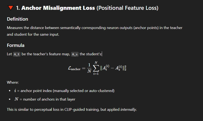
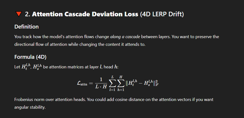
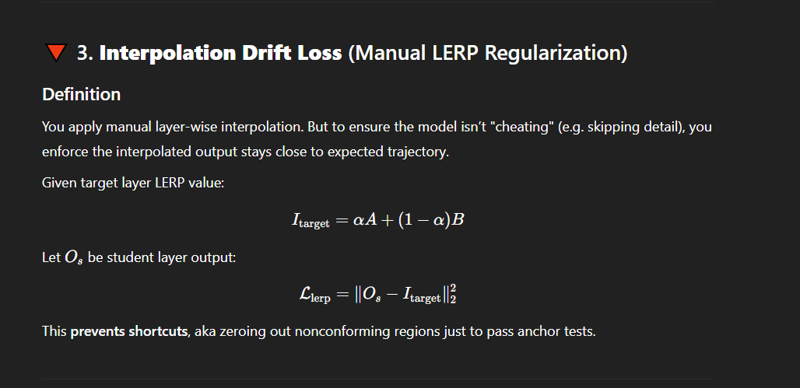
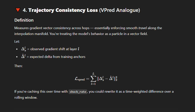
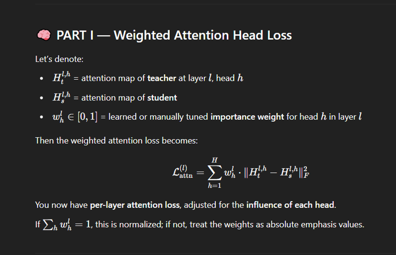
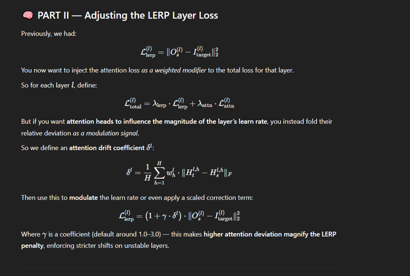
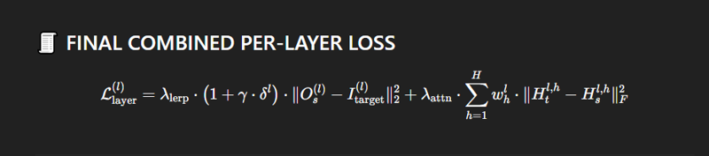
Loss
I really suck at formulating this sort of shit in terms of traditional math sense unless I'm in the very immediate spectrum and on some serious Adderall depth binge.
So this morning I fed it into GPT instead of trying to remember how I set it all up. I'll need to check the outcome later, but it's probably at least somewhat similar.