
Hello all,
Wolfgang Black here - a member of the ML/AI team here at Civitai. Welcome to the final installment of Machine Learning Projects: Classifying Content into Ratings. For those of you who have been following along, this is the final article! We finally made it to the multimodal models! I appreciate you all sticking around for the whole series! For anyone who's just getting introduced to this series - feel free to check out the article series for the background, or read on a head and let me know what ya'll think! In this series, we've been discussing how we've tackled the problem of trying to classify images and other media into movie-like ratings for our users to browse.
Despite this series detailing the work we've done for media classification, I wouldn't call this a solved problem! I've talked with other machine learning (ML) scientists at various social media companies who have expressed frustrations at existing ML solutions. The truth of the matter is, human moderators are needed across all levels and forms of media. Even at Civitai, we're still demoing this work in the backend as we try to tune our models to achieve better performance for labeling media.
This series of articles is to share insight with our efforts at Civitai and their results, especially since the deployment of these solutions may very well affect the site! Across the whole article series, I’ve had some great conversations and insights from our readers, so I invite that again below. Have ideas on how to tackle this problem? Want to try it on your own? Check out the dataset and engage in the comments, let's discuss!
In the previous articles we’ve shared how we’ve tackled the dataset capturing and the nuances of how to label data that is inherently difficult and can reflect personal views for a community, we discussed the single modality Computer Vision (CV) and Natural Language Processing (NLP) models we explored, all of which brings us to our mixture and multimodal efforts. These efforts seek to combine the single modality architectures either through voting or by utilizing the single modality model outputs as features for a Multi-Layer Perceptron (MLP).
As we showed in previous articles, this problem really lends itself to these kinds of multimodal solutions. The majority of images shared on Civitai were either generated with our onsite generator or uploaded to a user's profile after they generate the image locally. In most cases, users share the generation information - specifically the prompt used in generation. We also use ML models, like WD Tagger, to add tags to our media. Because of this we have two types of text data and the image data itself. To tackle this problem, we tried two main solutions: a mixture of 'experts' and a multimodal model. These models are composite solutions which take in the outputs of the hidden layers of other ML models. To create those solutions, we needed to do some traditional deep learning (DL) using our single modalities.
Like the previous modeling articles, this article will cover the models we explored, their architectures, and how these models performed. I'll try to include some images and tables, and I'll also link references when important. This isn't meant to be super instructive or to help people unfamiliar with the models master the concepts. It's more a project roadmap of how I tackled this problem. I'm always happy to discuss in the comments if there are questions. Before we get into the models though, let's remind ourselves what we're talking about at a high level.
Have you been following this work for a while? Feel free to skip to the good stuff - check out the Multimodal Systems - Mixtures and Multimodal Models section!
What are we trying to solve
At Civitai we receive hundreds of thousands of images from either our generation pipeline, where users experiment with different checkpoints and LoRAs, or ingestion from users sharing their locally generated images. We also receive a ton of data from users in training data sets, which users can use to create their own LoRAs onsite. When users want to make this data public and share with the community, we at Civitai have to make sure we can serve those images up to the appropriate audience. One way we do this is with image ratings that mimic movie ratings. Users are able to control the nature of the content they’ll see in their image by toggling on or off specific ratings.
To keep our users' browsing experience pleasant, we want our ratings to be accurate and representative of the content. Currently we use a system of tags, we rate the tags with a numeric value, and then determine a max allowable threshold per rating. If tags push the numeric value over a specific rating threshold, the rating graduates to a more restrictive level. However, we’re interested in trying to see if we can’t develop a machine learning system rather than a tagger fed algorithm to determine the rating. As such, I’ve tried a few different architectures, modalities, and strategies to build an end-to-end pipeline to correctly classify content with movie ratings
To approach this problem, we built mixture models which contain an odd number of single modalities and implement a voter layer. The single modality models each individually classify either the image or text. The text could be just the prompt or the prompt with the ML Tags. The models would classify their assigned modality and pass their prediction to the voter, which would select the most voted upon index. If there was a tie the more conservative, that is higher nsfw level, of the tie would be selected. We also experimented with multimodal models, which would take the pre-logit layers from different ML models and concatenate the outputs. These outputs would become the inputs of a simple MLP. This MLP would then output logits, which we'd select the highest logit to determine which classification of the media. Readers should know that the multimodal model requires more training, as each individual model was trained for our task and then the MLP was also further trained.

Multimodal Systems - Mixtures and Multimodal Models
In our quest for a multimodal solution that minimizes computation costs and GPU memory requirements, we first attempted to solve this problem with a pseudo-multimodal architecture - the mixture. A mixture model, sometimes referred to as a mixture of ‘experts’, combines different architectures to process various data modalities, creating a more discriminative output.
Mixture models are a family of models which have a specific area of expertise that can be either across a specific modality or for portion of the distribution within a single modality. They're closely related to ensemble methods, in which calculations are either performed multiple times or as a part of a study to create a probability distribution that represents the real world. As an aside, I have a computational physics background and I’m well acquainted with ensemble methods for simulating real world physics. It’s likely why I was drawn to experimenting with mixtures for this work - even though true multimodal models have shown great success in recent times and are only slightly more computationally expensive.
To create the mixture models, we utilized the various single model architectures, each processing its specific modality (e.g., text or image) to produce individual outputs. These outputs, which were the classifications each model made for the content, were then combined using a voting function. To ensure fairness, we used an odd number of diverse models in each mixture. In mixtures with 5+ models, any ties were resolved by selecting the more conservative category to prevent down-class misclassifications.
Mixtures have been used to combine various modalities or disparate data types in clustering, topic analysis, or as a mixture of experts with a gating network. This last method is most similar to what we’ve done here, but instead of a gating network we’ve utilized a voter function. Another difference between methods is that we did not change the datasets, outside of the ResNet50-CV which saw different slices of the same training data.
The natural evolution of these mixtures was to create a true multimodal model, as they’re known in modern ML. Multimodal models are incredibly powerful and have captured the attention of scientists and engineers in recent times. These architectures have contributed to systems and improved performance on text generation, captioning, image and video generations and will impact many industries in the coming years.
These models take networks with different modalities and use either a learned presentation of their outputs, some soft probabilities representing their outputs, or the final layer prior to predictions as inputs. This allows the combination of various model outputs, each with their own unique modality, through concatenation, as inputs to a new smaller network.. For example, if we have text embeddings E_t and image embeddings E_i, a multimodal model might use [E_t; E_i] as input to a final classifier.
These multimodal models often have simple feedforward networks or MLPs used to learn how to predict classes based on these concatenated inputs. These MLPs are smaller neural networks, often just a few layers of fully connected layers that step down with reasonable size from the input dimensions to the final prediction dimensions. In our case we’ve utilized drop out in our network to prevent overfitting.
An example of these network architectures was shown above, and we can see the main difference between the mixture and multimodal models is that the mixtures rely on accuracy of each individual model whereas the multimodal models rely on the base models learning representations of each class properly. Mixtures require slightly less training and are more model dependent. That is, once a model is trained with enough data as required by its architecture and training procedures it is ready to be used in a mixture. However, for a multimodal model even if each single modality model is well trained - we still need to train the multimodal model MLP itself.
One area of research we’re still working with here is the differences in data distribution between the MLP and the base models. That is, should we train on different examples? How much overlap should we have in each dataset for the CV, NLP, and MLP models? Have any ideas or want to discuss this theory? Let me know in the comments!
Now that we know what our multimodal systems look like, we should refresh ourselves on our single modality efforts. Below are the combined results of our CV and NLP models. The background on these models can be found in their respective articles, but for clarity and discussions sake we’ll share the models performances for accuracy, f1 score, and down class misclassification below.
Single Modality Model Results
We won't go into all the details of our CV and NLP efforts - for those readers should check out the previous articles. However, we wanted to remind readers of the models' performances on the classification tasks as these helped shape our multimodal experiments. During our CV model training, we explored the ResNet architecture as a baseline. Partnering with Pitpe11, a member of the community, we also utilize two different YOLO architectures and the canonical vision transformer - stepping from simple to complex model architectures. For this article, we’ll focus on two ResNet 50s, one trained with cross-validation; a Yolo trained for classification; and the vision transformer. For NLP, we focused our work mostly on lightweight DistilBerts and a RoBERTa - varying batch size and whether we included the tag text data.
To fairly compare the models we compared like modalities across accuracy, f1 score, and Down Class Misclassification (DCM), a significant metric for this project as it highlights the misclassification of images with significant differences in content rating like an X rated image being scored as PG13. Readers should note that we’re mostly concerned with the models ability to label R, X, and XXX correctly and not as PG or PG13. This line can also be considered the SFW-NSFW boundary.
The metrics we'll report out are derived metrics based on four parameters: True Positive (TP), False Positive (FP), True Negative (TN) and False Negative (FN). These concepts make up the base confusion matrix. To explain these concepts - let's consider a binary classifier which predicts class 0 or class 1. If the model predicts class 0 correctly, then we can say the model has made a TP prediction for class 0 - and a TN for class 1. If it predicts class 1 instead, it's a FN for class 0 and a FP for class 1. Thus every prediction falls into one of these categories across all classes. However, rather than considering each parameter for all classes we use summarized metrics. Below is a table with these summarized metrics and their definitions.


Experiments
For our mixture experiments we varied the number of models, the mixture compositions, and weighing different modalities or models in the voting layer. Our experiments in multimodal modeling were similar in that we explored the number of models, the compositions of the inputs, but we also explored training the MLP with different loss functions.
Below is a table showing the different mixture and multimodal models and their compositions. While we explored many more compositions than these, we tried to use the single modal model performances as a north star for building the compositions. We focused specifically on what models performed well on DMC and f1 scores for R and PG. For the mixtures we leaned heavily on the top performing models and looked at their DMC graphs, graphs of images each model mislabeled, to attempt to prevent all models missing the same important data. For the multimodal models, we also optimized for top f1 scores.

Readers will note early we didn’t share any results from the ResNet18 or Yolo-Det models. These results can be found in the CV article.
The second section of the table above shows the base name for the multimodal models. This base name indicates the computational requirements of the multimodal composition. However we ran over 20 experiments for the multimodal models varying loss functions, pretraining, model composition, cross validation, and more.
Below in the results section we’ll share results from the top three performing multimodal models - all of which use a slightly different loss function during training. While we have a multiclass problem, we’re more concerned with either the performance of identifying the True Positives and reducing the False Positives of PG, or the NSFW-SFW boundary - that is, properly identifying R. To try to emphasize ‘correctness’ on specific classes, we weighted these parameters either in the traditional loss function (Cross Entropy) or in the soft f1 loss function.
To prioritize a specific class using the cross entropy loss function, we found the loss associated with each label during training, and then either averaged the losses together or weighted them by some parameter, ⍺. The other parameters were then weighted by (1-⍺)/(n-1) where n is the number of classes total. So long as ⍺ > 0.2, the model would more heavily penalize the loss associated with the specific class.
We also utilize a soft f1 loss. By using this loss function we could attempt to optimize towards better macro f1 performance - the models ability to prioritize true positive labeling of the classes. This also gave us the ability to more heavily weight a specific class's F1 performance by ignoring the basic averaging of the f1s per class and assigning our specified class more weight, as described above. To do this, we had to treat the True/False Positives/Negatives as continuous sums as opposed to discrete integers. Doing this allowed us to calculate the f1-score as though it were differentiable. From there we could replace the cross-entropy loss function.
To denote the models and their specific loss functions, we’ll use the suffixes in the following format: model-CLASS-weight-metric. Here the class will be either PG or R; weight will be either ‘W’ (denoting greater weight on the class metric) or N meaning non-weighted; and metric will be either f1 or loss. If f1, we’ll utilize a soft f1 loss function, otherwise we’ll utilize the standard loss function. Readers should note that if the weight field is N meaning none, then the class specified doesn’t matter, as all classes are weighted evenly in the loss calculations.
Results
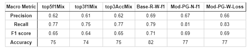
In this section we’ll go over the accuracy, f1, and DMC of the mixture and multimodal models. We’ll also share the macro performance of accuracy, precision, recall, and f1 for each of the multimodal models. One could calculate the macro performance for accuracy and f1 for all the models presented here if motivated, though that macro performance may differ slightly due to the small variation in samples per class.
The first table we’ll look at is the class specific accuracy per model. In this table we see that generally multimodal models perform better than mixtures, in some cases having over 10 points over their mixture counterparts. The real power of these multimodal techniques can be seen in R with Base-R-W-f1 and Mod-PG-W-Loss showing a significant increase of over 15 points relative to the single modal models and the mixtures. While this is impressive, it comes at no cost to the neighboring classes - both of these models achieve over 70% and 90% accuracy for PG13 and X respectively. While all the presented multimodal systems achieved over 69% accuracy and over 85% accuracy in PG13 and R respectively, the single modal models largely struggled with these intermediate classifications.

Just like in the class accuracy we see that the multimodal models largely out perform their mixture counterparts across every class. It’s also incredible to see the f1s for XXX and X approach 1, though the PG f1 scores are lower than we’d like. However, this might be centered around misclassifications of PG-PG13 and may not be catastrophic. To check this we can look at the DCM table.

true labels are actually wrong! The majority of the DMC XXX-PG and XXX-PG13 contain questionable labels, and actually spurred a relabeling effort that was started AFTER this work was finished. We wanted to keep all the data the same through the entire modeling project, so that we did not misrepresent any single model or multimodal model performance. A post mortem of the data revealed that even among the CV and NLP models some, but not all, of the misclassified NSFW-SFW images were actually mislabels and the models were correct in their predictions
Mislabels aside, the general performance of the multimodal models are better with fewer DMCs crossing the NSFW-SFW boundary. The exception to this rule is BASE-R-W-f1, which has the most DMCs in this study. However, this model also had the least XXX-PG, X-PG13, and X-R mislabels. It’s interesting to see that the Mod models have the least amount of DMCs, and that the standard weighted loss model Mod-PG-W-Loss performs better than the other models with around 30% fewer DCMs when compared to the mixtures and the Base multimodal model.


Finally when we consider the performance of the multimodal models holistically like this we see that on this evaluation test set we have the best performance in the Base-R-W-f1 model, with a whooping 82% accuracy and .71 macro f1 score. Reaching this level of performance we’ve now started testing these models in the backend and are trying to surface the classifications to our moderator team to determine if the models are ready for site-community interactions.
 Conclusion
In this work we’ve presented our efforts towards trying to classify media containing text and images, into movie like classifications. We sourced labeled data by engaging with the community who labeled images on a scale of PG-XXX, representing family-friendly to explicitly nsfw. This data was then compared to a key, and false or poorly mislabeled data was removed to prevent bad actors or community members with very different ratings from manipulating the data in ways that would violate our original goals and terms of service. To get the final dataset we took examples that had 3 or more votes, found the more conservative highest voted rating per image, and then stored the image alongside its prompts and tags. The tags, used onsite for filtering and searching, were generated by the WD Tagger model popular in the community.
The data was split into a training and validation set. The training data had some 21k examples with relatively even samples across the 5 classes. The evaluation set was then supplemented with moderator sourced data to create an evaluation set of some 12images - this set was not balanced. The training data can be found <here>.
After the data capture step, we researched performance of single modality models. We utilized simple to complex ML and DL models in an attempt to understand whether we had enough data to capture the trends and distributions necessary to be performant in a live example, and to understand the computational complexity of each model.
We experimented with three computer vision methods, using various techniques to process the data and train the models. Here we found that the models performed similarly on the PG and XXX classes, but that macro behavior and DCM could be improved by more modern techniques. We also experimented with three NLP architectures, mostly leaning on modern transformers to try to solve this problem. Here we found that DistilBerts, a computational efficient architecture, performed very well especially with Tags - but that the larger RoBERTa method was slightly better in performance.
Once we had an idea of how the single modality models performed and their strengths, we ran a large factorial study on mixtures and multimodal models. The mixtures involved testing single modality models and comparing various compositions in a voter function. This testing style was computational efficient as each model was run one time and their outputs fed into the voter as a sort of post processing. These mixtures performed much better than a single modal model but still had the same weaknesses of having difficulty with the NSFW-SFW line and properly identifying the middle classes.
Finally, we explored using the single modality models as feature generators for a simple multilayer perceptron. This meant removing the classification layers from the various models and constructing a large architecture to process the text and image modalities into inputs fed into a smaller neural network. This network was further trained on the data, freezing the weights of the single modality models. These models performed even better on the tasks, scoring high marks in f1 scores and class accuracies.
The Next steps
Machine Learning, Deep Learning, AI - it’s all iterative. Throughout this series I've been engaging with the community and trying out their suggestions and ideas. Several community members have mentioned that the dataset is poorly labeled - we wanted to interfere as little as possible with the data labeled by the larger community, as the labels should reflect what our users want to see. However, we have come to notice some small percent of images in the training data that do indeed need to be relabeled.
We’re also going through our moderator sourced data used in the evaluation set and using this to expand the current training data. The near term goal is to expand the training data to be some 12k images per class. Similarly we’re checking out our most important classes of XXX, PG, and R in our evaluation sets to make sure our reported DCMs are more accurate in the future.
Community members have also pointed out newer transformers used in Vision. The BEiT model and ConvNext models are two more modern models that have significant improvements over the ViT. I’ve started to explore training these models and seeing if we can use these to shrink the footprint of the current multimodal models. Similarly, I'm looking at more modern text classifiers to see if we can’t find a more efficient method than calling both the DistilBert+Tags and the RoBERTa in our models.
While I casually explore other potential options to use in my multimodal models, we’re testing the multimodal models in the background - using the classifications in the backend and checking to see what grievous errors occur. We’ll also use this data to iterate and improve the models performance, so we can eventually use these tools on the front end and free up our moderators to deal with one of their other thousands of challenges!
For any community members who are interested, inference with these models currently requires 3.5 GB of GPU memory - so the goal is to increase performance over the metrics shared above while either maintaining or lowering this footprint. We want a modern solution which we can host ourselves with little cost and latency.
This concludes our series on classifying content into ratings using multimodal models. I want to thank everyone who has followed along and engaged with this work. Your input has been invaluable, and I'm excited to continue this collaborative approach as we refine our models and explore new directions.
For those just joining us, I encourage you to explore the earlier articles in this series for a comprehensive understanding of our journey. Whether you're curious about the intricacies of ML models, interested in dissecting diffusion models, or simply want to learn more about our moderation and generation projects at CivitAI, I'm here to help. Please share your thoughts, questions, or suggestions in the comments below or reach out to me directly on the site.
As we take a brief pause in our ML team's article series, I'm eager to hear what topics you'd like us to cover next. Your feedback will shape our future content, ensuring we address the areas that most interest and benefit our community. Together, we can continue to improve content searching, sharing, and viewing on Civitai, making it an even better platform for all users.
Stay tuned for more exciting developments, and don't hesitate to engage with us. Your insights and curiosity drive our work forward, and I look forward to our ongoing dialogue about the fascinating world of AI and machine learning